What has Edge of Stability to do with the Convergence Theory?

Edge of Stability

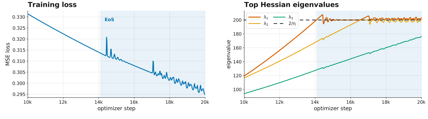
A full-batch gradient-descent MLP trajectory on CIFAR-10. Left: training loss decreases monotonically until the top Hessian eigenvalue reaches the stability threshold, then oscillates while continuing to decrease. Right: the top three Hessian eigenvalues, with lambda one and lambda two approaching the dashed two-over-stepsize threshold. The post-crossing EoS region is shaded blue in both panels.

2-layer tanh MLP · CIFAR-10 · full-batch GD · MSE · \eta=0.01.

w_{t+1}=w_t-\eta\nabla {\color{#0072B2}{f(w_t)}}.

2-layer tanh MLP · CIFAR-10 · full-batch GD · MSE · \eta=0.01.

w_{t+1}=w_t-\eta\nabla {\color{#0072B2}{f(w_t)}}.

{\color{#D55E00}{\mathcal S(w_t)}} := {\color{#D55E00}{\lambda_{\max}}}\!\left(\nabla^2 f(w_t)\right).

{\color{#D55E00}{\mathcal S(w_t)}} \approx {\color{#171717}{\frac{2}{\eta}}}.

Modern deep learning typically operates at the Edge of Stability.

Cohen et al. (2021), Gradient Descent on Neural Networks Typically Occurs at the Edge of Stability.

The EoS phase can occupy most of LLM pretraining

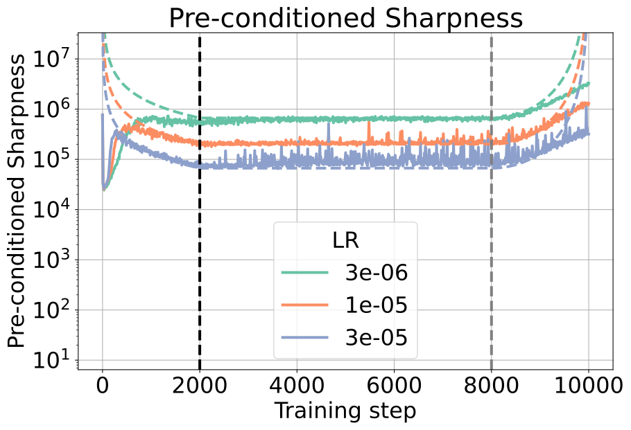
Measured sharpness · ∼100M GPT-style Pre-LN · FineWebEdu-10B · AdamW · WSD

WARMUP

STABLE

DECAY

Constant-LR phases dominate pretraining of LLMs

Laguna XS.2≈70% near peak LR final 30% is decay; warmup length not reported

Nemotron 3 Ultra74% stable1% warmup · 25% decay

DeepSeek-V4-Pro>50% at peak LR†† conservative lower bound; exact decay share not reported

Kalra et al. (2026), Fig. 4a (source panel; CC BY 4.0). Schedules: Poolside, NVIDIA & DeepSeek-AI (2026).

The quadratics

f(x)=\frac12 x^\top Hx, \qquad H\succeq0, \qquad \lambda_{\max}(H)=L.

{\color{#0072B2}{ \begin{gathered} 0<\eta<\frac{2}{L}, \\[0.55em] \lambda_{\max}(H)=L<\frac{2}{\eta}, \\[0.55em] f(x_{t+1})<f(x_t), \qquad x_t\longrightarrow0. \end{gathered} }}

{\color{#E69F00}{ \begin{gathered} \eta=\frac{2}{L}, \qquad x_0\parallel v_{\max}, \\[0.55em] \lambda_{\max}(H)=L=\frac{2}{\eta}, \\[0.55em] x_{t+1}=-x_t, \qquad f(x_{t+1})=f(x_t). \end{gathered} }}

{\color{#D55E00}{ \begin{gathered} \eta>\frac{2}{L}, \qquad \langle x_0,v_{\max}\rangle\ne0, \\[0.55em] \lvert1-\eta L\rvert>1, \\[0.55em] \lVert x_t\rVert\longrightarrow\infty, \qquad f(x_t)\longrightarrow\infty. \end{gathered} }}

Expectation vs Reality

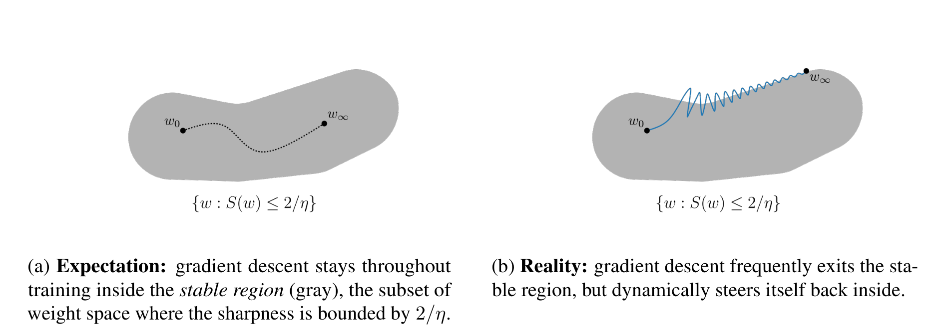
Figure 4 from Cohen et al. contrasting the traditional expectation that gradient descent remains inside the stable region with the reality that it repeatedly exits and dynamically returns.

Classic optimisation theory

Reality

Cohen et al. (2025), Figure 4(a–b).

Edge of Stability timeline

OBSERVE

precursorsWu–Ma–E ’18
Jastrzębski et al. ’19, ’20
Lewkowycz et al. ’20

full-batch EoSCohen et al. ’21

adaptive / stochasticCohen et al. ’22
Lee–Jang ’23
Andreyev–Beneventano ’24

geometry / scaleIslamov et al. ’26
Kalra et al. · Cai et al. ’26
Meterez et al. ’26

MODEL

unstable GDArora et al. · Ahn et al. ’22

progressive sharpeningLi et al. ’22
Agarwala et al. · Zhu et al. ’23

reduced dynamicsChen–Bruna ’23

continuous flowsCohen et al. ’25
Regis–Chewi · Marion ’26

EXPLAIN

self-stabilizationDamian et al. ’23

origin / alignmentLowell–Kastner ’24
Litman ’26

dominant / bulkSong et al. ’25

product / bifurcationGan et al. ’26a,b

CONSEQUENCES

implicit biasWu et al. · Even et al. ’23
Fojtik et al. ’25

overparametrized LS ratesMacDonald et al. ’25

curvature-aware tuningRoulet et al. ’24

generalizationTuci et al. ’26

QUESTION: What drives convergence at the Edge of Stability?

{\color{#9A5F37}{\mathcal S(w):=\lambda_{\max}}}\!\left(\nabla^2 f(w)\right)

But it is the wrong variable for observing convergence.

Setting

{\color{#3E7786}{g_t}}:=\nabla f(x_t),\qquad x_{t+1}=x_t-\eta {\color{#3E7786}{g_t}}.

{\color{#56B4E9}{\bar{\lambda}_t}} := \frac{ {\color{#3E7786}{g_t}}^\top \left(2\!\int_0^1(1-\tau)\nabla^2 f(x_t-\tau\eta {\color{#3E7786}{g_t}})\,d\tau\right) {\color{#3E7786}{g_t}} }{\lVert {\color{#3E7786}{g_t}}\rVert^2}

= \frac{2}{\eta} + \frac{2\bigl[f(x_{t+1})-f(x_t)\bigr]} {\eta^2\lVert {\color{#3E7786}{g_t}}\rVert^2}

Directional sharpness (Roulet et al., 2024)

f\in C^2(\mathbb R^d), \qquad {\color{#78647D}{\Delta_t}} :=x_{t+1}-x_t =-\eta {\color{#3E7786}{g_t}}.

f(x_{t+1})-f(x_t) \overset{\mathrm{Taylor}}{=} {\color{#3E7786}{g_t}}^\top {\color{#78647D}{\Delta_t}} + \int_0^1(1-\tau)\, {\color{#78647D}{\Delta_t}}^\top\nabla^2 f(x_t+\tau {\color{#78647D}{\Delta_t}}){\color{#78647D}{\Delta_t}}\,d\tau.

\begin{aligned} f(x_{t+1})-f(x_t) &= -\eta\lVert {\color{#3E7786}{g_t}}\rVert^2 + \eta^2\!\int_0^1(1-\tau)\, {\color{#3E7786}{g_t}}^\top\nabla^2 f(x_t-\tau\eta {\color{#3E7786}{g_t}}){\color{#3E7786}{g_t}}\,d\tau \\[0.55em] &= -\eta\lVert {\color{#3E7786}{g_t}}\rVert^2 + \frac{\eta^2}{2}\lVert {\color{#3E7786}{g_t}}\rVert^2 {\color{#56B4E9}{\bar{\lambda}_t}}. \end{aligned}

f(x_{t+1})-f(x_t) = -\eta\, \underset{{\color{#3E7786}{\text{gradient energy}}}}{ {\color{#3E7786}{\boxed{\lVert g_t\rVert^2}}}} \qquad \underset{{\color{#557D66}{m_t\;\text{step margin}}}}{ {\color{#557D66}{\boxed{\left(1-\frac{\eta {\color{#56B4E9}{\bar{\lambda}_t}}}{2}\right)}}}}.

Timing: 3:55–5:15

For a nonzero gradient, apply Taylor’s formula along the actual update segment.

I will not read the entire integral. It is simply the exact Taylor remainder accumulated along the step from x_t to x_t+1.

The averaged sharpness λ̄_t is the curvature in the gradient direction, averaged along this complete finite step.

For a quadratic, it reduces to the Rayleigh quotient

g_t^⊤Hg_t / ‖g_t‖².

For a nonlinear objective, the path average is essential because the learning rate is not infinitesimal at EoS.

Now define the step margin

m_t = 1 − ηλ̄_t/2.

The only identity to retain from this slide is

f(x_t+1) − f(x_t) = −η‖g_t‖²m_t.

This is exact; there is no approximation and no small-step assumption.

Consequently, λ̄_t < 2/η is equivalent to descent, while λ̄_t > 2/η is equivalent to a loss increase.

Moreover, λ̄_t can be computed from two consecutive losses and the gradient norm, without computing a Hessian eigenvalue.

Averaged sharpness decides descent; \lambda_{\max} does not

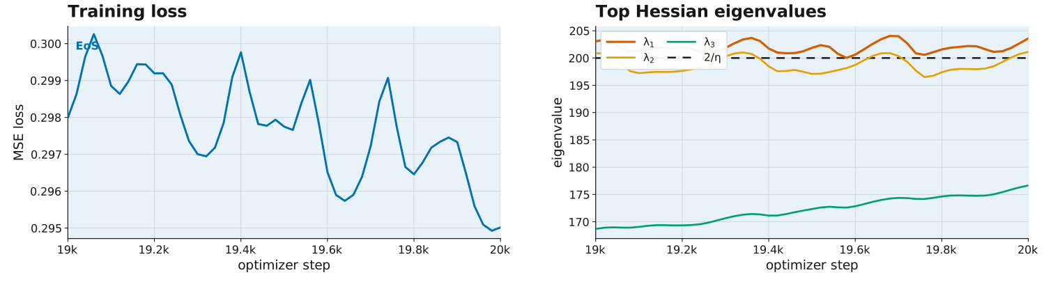
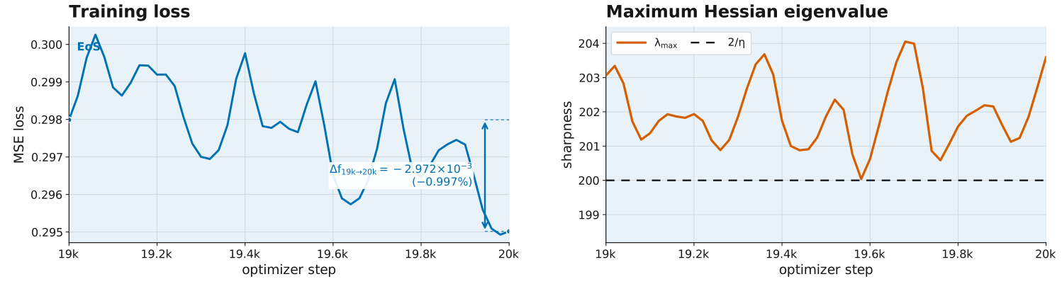
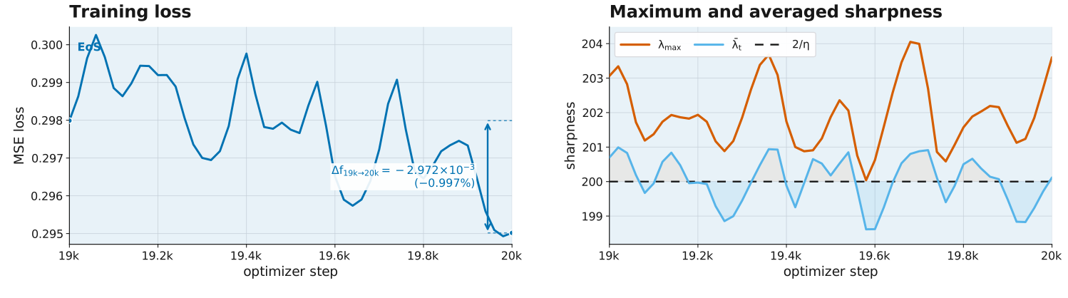
The same full late-training loss and top-three Hessian-eigenvalue trajectory shown on slide 2. The same loss and top-three eigenvalue plots zoomed to optimizer steps 19,000 through 20,000. The late-window loss and maximum Hessian eigenvalue. The loss drops by 0.997 percent although the maximum eigenvalue stays strictly above the stability threshold. The late-window loss, maximum Hessian eigenvalue, and averaged directional sharpness. Averaged sharpness oscillates around the stability threshold while the maximum eigenvalue remains above it.

-\eta\lVert g_t\rVert^2 \left(1-\frac{\eta{\color{#D55E00}{\lambda_{\max}(H_t)}}}{2}\right)>0, \qquad {\color{#D55E00}{\lambda_{\max}(H_t)}}>{\color{#171717}{\frac{2}{\eta}}} \quad\not\Rightarrow\quad f(x_{t+1})-f(x_t)>0.

\begin{gathered} {\color{#56B4E9}{\bar{\lambda}_t}} = \frac{2}{\eta} + \frac{2\bigl[f(x_{t+1})-f(x_t)\bigr]} {\eta^2\lVert g_t\rVert^2}, \\[0.55em] {\color{#56B4E9}{\bar{\lambda}_t}} > {\color{#171717}{\frac{2}{\eta}}} \quad\Longleftrightarrow\quad f(x_{t+1})-f(x_t)>0. \end{gathered}

The top eigenspace can stall while the bulk still descends

g_t:=\nabla f(x_t), \qquad H_t=\sum_{i=1}^{d}\lambda_i(t)u_i(t)u_i(t)^\top.

\lambda_1(t)\ge\cdots\ge\lambda_k(t) \ge \lambda_{k+1}(t)\ge\cdots\ge\lambda_d(t)

Dom-GD

\begin{gathered} P_{\mathrm{dom},t}:=\sum_{i=1}^{k}u_i(t)u_i(t)^\top, \\[0.65em] {\color{#E69F00}{ x_{t+1}^{\mathrm{dom}}=x_t-\eta P_{\mathrm{dom},t}g_t. }} \end{gathered}

Bulk-GD

\begin{gathered} P_{\mathrm{bulk},t}:=I-P_{\mathrm{dom},t}, \\[0.65em] {\color{#009E73}{ x_{t+1}^{\mathrm{bulk}}=x_t-\eta P_{\mathrm{bulk},t}g_t. }} \end{gathered}

Song, Ahn & Yun, Does SGD Really Happen in Tiny Subspaces?, ICLR 2025.

Panel (a) · Toy model

\Phi(w_1,w_2,s)=(1-w_1w_2)^2+\frac{s^2}{2000}.

\eta=0.501 · (w_{1,0},w_{2,0},s_0)=(1,0.95,5) · k=1 · t_\star=25

Panel (b) · Neural network

Dataset CIFAR-10 · 50,000 train Loss MSE Model 2-layer tanh MLP · width 200

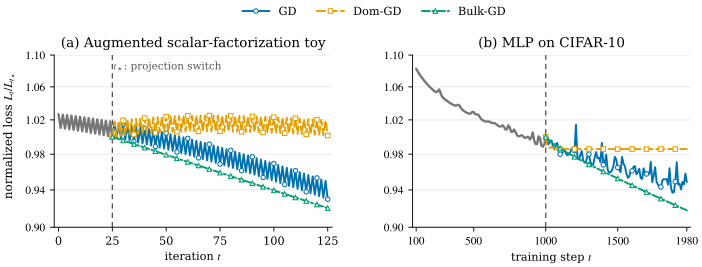
full-batch GD · \eta=0.05 · k=10 · t_\star=1000

Theory and neural-network experiments comparing full gradient descent, orange dominant-subspace gradient descent, and green bulk-subspace gradient descent. The augmented scalar-factorization toy and the CIFAR-10 MLP both show dominant updates stalling while bulk updates descend.

{\color{#E69F00}{\lambda^\eta_{\mathrm{dom},t}}} > \frac{2}{\eta} \approx {\color{#56B4E9}{\bar\lambda_t}} > {\color{#009E73}{\lambda^\eta_{\mathrm{bulk},t}}} \quad\overset{\mathrm{observed}}{\Longrightarrow}\quad {\color{#E69F00}{f(x_T^{\mathrm{Dom}})}} > {\color{#0072B2}{f(x_T^{\mathrm{GD}})}} > {\color{#009E73}{f(x_T^{\mathrm{Bulk}})}}.

Song, Ahn & Yun, Does SGD Really Happen in Tiny Subspaces?, ICLR 2025.

Timing: 5:55–6:50

A second and orthogonal example comes from dominant-versus-bulk gradient descent.

Dominant GD projects the gradient onto the leading Hessian eigenspace. Bulk GD uses the complementary subspace. At the switching point, these two projected updates decompose the full gradient update.

After switching from full GD, the dominant method stalls. The bulk method continues to descend smoothly and can even outperform full GD. This occurs both in the theoretical toy model and in the neural-network experiment.

The observed ordering is

λ_dom,t > 2/η ≈ λ̄_t > λ_bulk,t,

which is consistent with the corresponding ordering of final losses.

The conclusion is not that the top eigenspace never matters. It is that the worst-curvature subspace can carry little useful progress, while the bulk carries most of the descent.

Multi-step convergence at EoS

{\color{#557D66}{M^g_{s:T}}} := \frac{ \sum_{t=s}^{T-1}{\color{#3E7786}{\lVert g_t\rVert^2}}{\color{#557D66}{m_t}} }{ \sum_{t=s}^{T-1}{\color{#3E7786}{\lVert g_t\rVert^2}} }

{\color{#557D66}{m_t}} := 1-\frac{\eta {\color{#56B4E9}{\bar{\lambda}_t}}}{2}.

f(x_t)-f(x_{t+1}) = \eta\,{\color{#3E7786}{\lVert g_t\rVert^2}}\,{\color{#557D66}{m_t}}.

\sum_{t=s}^{T-1}\bigl[f(x_t)-f(x_{t+1})\bigr] = \eta\sum_{t=s}^{T-1} {\color{#3E7786}{\lVert g_t\rVert^2}}\,{\color{#557D66}{m_t}}.

f(x_s)-f(x_T) = \eta {\color{#557D66}{M^g_{s:T}}} \sum_{t=s}^{T-1}{\color{#3E7786}{\lVert g_t\rVert^2}}.

\boxed{ f(x_T)<f(x_s) \quad\Longleftrightarrow\quad {\color{#557D66}{M^g_{s:T}}}>0 }

A positive EoS margin restores convergence rates

Theorem.

\begin{gathered} f\in C^2(\mathbb R^d),\qquad x_{t+1}=x_t-\eta g_t,\qquad g_t=\nabla f(x_t),\qquad \eta>0,\qquad 0\le s<T. \end{gathered} {\color{#557D66}{m_t}}:=1-\dfrac{\eta{\color{#56B4E9}{\bar\lambda_t}}}{2}, \qquad {\color{#557D66}{M^g_{s:T}}} := \dfrac{\sum_{t=s}^{T-1}{\color{#3E7786}{\lVert g_t\rVert^2}}{\color{#557D66}{m_t}}} {\sum_{t=s}^{T-1}{\color{#3E7786}{\lVert g_t\rVert^2}}}. {\color{#557D66}{M^g_{s:T}}} \ge {\color{#557D66}{\gamma_{\eta,T-s}}}>0.

(iii) Polyak–Łojasiewicz condition.

\begin{gathered} \textbf{Assume}\quad \mu>0,\quad \mathcal X_\star\ne\varnothing,\quad \lVert\nabla f(x)\rVert^2\ge2\mu\bigl(f(x)-f_\star\bigr), \\[0.65em] \textbf{Then} \\[0.15em] \frac1{T-s}\sum_{t=s}^{T-1}\bigl(f(x_t)-f_\star\bigr) \le \frac{f(x_s)-f_\star} {2\mu(T-s){\color{#557D66}{\gamma_{\eta,T-s}}}}. \end{gathered}

Timing: 7:45–8:55

First reveal the finite-horizon assumptions and the positive margin condition. Then reveal the PL consequence.

Suppose that the weighted margin on a horizon of length T − s is bounded below by a positive quantity

M^g_s:T ≥ γ_η,T−s > 0.

Under the Polyak–Łojasiewicz condition,

½‖g_t‖² ≥ μ(f(x_t) − f_★),

the accumulated gradient energy controls the average function-value gap. Combining this with the exact identity gives the displayed bound.

If γ_η,T−s scales as (T − s)^−α, the average suboptimality scales as (T − s)^−(1−α).

The convergence problem at EoS is therefore reduced to one question:

How large a positive lower bound can we prove for the realized horizon margin?

The theorem itself is deliberately elementary. The substantive work is deriving the margin bound from the dynamics.

The general non-convex, aiming-condition, and blockwise PL guarantees are in the backup slides.

The EoS-simulating toy model

F(w_1,w_2):=(y-xw_1w_2)^2,\quad x,y>0,\quad \rho:=\frac yx,\quad w_0=\sqrt{\rho}\,(1,1-h),\quad h\in\left(0,\frac12\right),\quad \eta=\eta_c:=\frac1{2xy}.

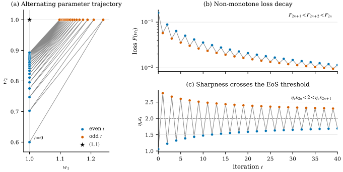
Trajectory, loss, and normalized sharpness for gradient descent on the scalar factorization model. The iterates zigzag toward the minimizer, loss decreases over each two-step cycle, and sharpness crosses the EoS threshold at every step.

{\color{#0072B2}{F_{2n+1}}} < {\color{#0072B2}{F_{2n+2}}} < {\color{#0072B2}{F_{2n}}}, \qquad F_t\longrightarrow0.

\eta_c{\color{#D55E00}{\kappa_{2n}}}<2< \eta_c{\color{#D55E00}{\kappa_{2n+1}}}, \qquad \eta_c{\color{#56B4E9}{\bar\lambda_{2n}}}<2< \eta_c{\color{#56B4E9}{\bar\lambda_{2n+1}}}.

{\color{#557D66}{M^g_{0:T}}} \ge \frac{h^2}{16[1+\log(1+2Th^2)]} = \Omega\!\left(\frac1{\log T}\right).

\lVert\nabla F(w_t)\rVert^2 \ge 2{\color{#78647D}{\mu_h}}F(w_t), \qquad {\color{#78647D}{\mu_h}} := 2xy\!\left[1+(1-h)^2\right].

\frac1T\sum_{t=0}^{T-1}F(w_t) \le \frac{F(w_0)} {2{\color{#78647D}{\mu_h}}\,T\,{\color{#557D66}{M^g_{0:T}}}} = O\!\left(\frac{\log T}{T}\right), \qquad \min_{0\le t<T}\lVert\nabla F(w_t)\rVert^2 = O\!\left(\frac{\log T}{T}\right).

Timing: 8:55–10:15

Let us test this reduction on the smallest model reproducing the phenomenon.

This is a two-parameter factorized least-squares objective,

F(w₁,w₂) = (y − xw₁w₂)²,

initialized close to its minimizer manifold and run at the critical step η_c.

The trajectory has a parity-two structure.

One step decreases the loss. The following step increases it. Nevertheless, every complete two-step block makes net progress.

At the same time, the averaged sharpness alternates below and above 2/η. Thus the model reproduces persistent loss oscillations in exactly the quantity that controls the one-step change.

For this trajectory, the gradient-energy-weighted margin remains positive and admits a lower bound of order

M^g_0:T = Ω(1/log T).

Combining this with a PL inequality on the invariant region visited by the iterates gives

(1/T) ∑_t=0^T−1 F(w_t) = O(log T / T),

and

min_0≤t<T ‖∇F(w_t)‖² = O(log T / T).

The message is that loss spikes do not preclude a deterministic convergence rate. They weaken the effective margin.

Higher-order EoS toy model: cross-entropy

\begin{gathered} r:=w_1w_2-1,\qquad F_{\mathrm{CE}}(w_1,w_2):=\log 2+\log\cosh\!\left(r+\frac13r^3\right),\qquad F_{\mathrm{CE}}^\star=\log2,\\[-0.12em] w_{1,0}=w_{2,0}=\sqrt{1-h},\qquad 0<h\le h_0,\qquad \eta_c=1. \end{gathered}

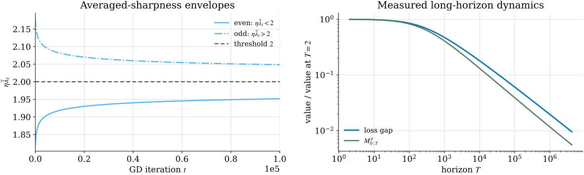
Exact cross-entropy higher-order toy-model dynamics. Averaged sharpness alternates across the threshold for one hundred thousand steps, while the measured loss gap and cumulative margin decay through horizon two to the twenty-second power.

\eta_c{\color{#56B4E9}{\bar\lambda_{\mathrm{CE},2n}}}<2< \eta_c{\color{#56B4E9}{\bar\lambda_{\mathrm{CE},2n+1}}},\qquad \eta_c{\color{#56B4E9}{\bar\lambda_{\mathrm{CE},t}}}\longrightarrow2.

{\color{#0072B2}{F_{\mathrm{CE},t}-F_{\mathrm{CE}}^\star}} = \Theta_h\!\left(t^{-1/2}\right).

\begin{gathered} {\color{#0072B2}{F_{\mathrm{CE},t}-F_{\mathrm{CE}}^\star}} =\Theta_h\!\left(t^{-1/2}\right),\\[-0.05em] {\color{#557D66}{M^{g,\mathrm{CE}}_{0:T}}} \ge \dfrac{h^4}{1024\!\left[1+\left(\frac85Th^4\right)^{1/2}\right]} =\Omega_h\!\left(T^{-1/2}\right). \end{gathered}

Higher-order EoS toy model: mean squared error

\begin{gathered} r:=w_1w_2-1,\qquad F_{\mathrm{MSE}}(w_1,w_2):=\frac12r^2+\frac14r^4,\qquad F_{\mathrm{MSE}}^\star=0,\\[-0.12em] w_{1,0}=w_{2,0}=\sqrt{1-h},\qquad 0<h\le h_0,\qquad \eta_c=1. \end{gathered}

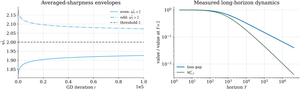
Exact mean-squared-error higher-order toy-model dynamics. Averaged sharpness alternates across the threshold for one hundred thousand steps, while the measured loss gap and cumulative margin decay through horizon two to the twenty-second power.

\eta_c{\color{#56B4E9}{\bar\lambda_{\mathrm{MSE},2n}}}<2< \eta_c{\color{#56B4E9}{\bar\lambda_{\mathrm{MSE},2n+1}}},\qquad \eta_c{\color{#56B4E9}{\bar\lambda_{\mathrm{MSE},t}}}\longrightarrow2.

{\color{#0072B2}{F_{\mathrm{MSE},t}-F_{\mathrm{MSE}}^\star}} = \Theta_h\!\left(t^{-1/3}\right).

\begin{gathered} {\color{#0072B2}{F_{\mathrm{MSE},t}-F_{\mathrm{MSE}}^\star}} =\Theta_h\!\left(t^{-1/3}\right),\\[-0.05em] {\color{#557D66}{M^{g,\mathrm{MSE}}_{0:T}}} \ge \dfrac{h^6}{512\!\left[1+\left(60Th^6\right)^{2/3}\right]} =\Omega_h\!\left(T^{-2/3}\right). \end{gathered}

Empirical EoS margin scaling law

ViT · CIFAR-10k · full-batch GD · CE and MSE · 10 learning rates · 10–11 seeds / rate

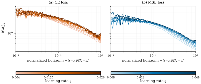
Cumulative weighted EoS margin dynamics for ViT training on CIFAR-10k with cross-entropy and mean-squared error across learning rates and seeds.

N:=T-s,\qquad {\color{#557D66}{M^g_{s:s+N}}} \gtrsim {\color{#557D66}{cN^{-\widehat\alpha}}},\qquad {\color{#557D66}{\widehat\alpha}}\le\frac12.

Conclusions

\lambda_{\max} does not describe convergence at EoS.

Toy models help us understand the phenomenon.

Despite loss spikes, we find statistically significant evidence of polynomial convergence at EoS.

The optimisation workflow

f_\theta

EoS-friendly, general toy models

\mathcal A_{\mathrm{EoS}}

Optimization assumptions that reproduce EoS dynamics

\operatorname{rate}(T)

Convergence guarantees

Promising directions

\mathcal M_{\mathrm{EoS}}

Structure of the EoS manifold

Initialization at EoS

\eta_t

EoS with learning-rate schedules

\mathrm dX_t

Stochastic EoS

SDE / gradient-flow limits

Backup slides

Five-minute question preparation

1. Is the margin assumption circular? You define M^g_s:T using the observed decrease.

At the identity level, M^g_s:T is indeed an ex-post quantity. The theorem should be understood as a reduction theorem, not as the complete convergence theory. It identifies progress per unit accumulated gradient energy as the missing object. The nontrivial part is to derive a lower bound on this margin from structural properties of the dynamics. The toy models do exactly this: their margin lower bounds are proved directly from the recursion, rather than assumed after observing convergence.

It is analogous to identifying the correct Lyapunov drift. Writing the drift is elementary; proving that it remains positive is the substantive result.

2. Why not use the pointwise directional curvature g_t^⊤∇²f(x_t)g_t/‖g_t‖²?

Because the step at EoS is not infinitesimal. The exact Taylor remainder depends on the Hessian along the entire segment from x_t to x_t+1. The pointwise Rayleigh quotient is only a small-step approximation. For a quadratic, where the Hessian is constant, the two quantities coincide.

3. Are you claiming that λ_max is useless?

No. It remains a sufficient worst-case stability certificate and an important diagnostic of the geometry. The claim is only that it is not necessary for realized descent and does not determine the sign or rate of progress. It ignores both gradient alignment and variation of the Hessian along the finite step.

A uniform pathwise bound on λ_max still upper-bounds the averaged sharpness; it is sufficient, simply conservative.

4. Does oscillation of λ̄_t around 2/η imply convergence?

No. Oscillation alone is insufficient. The unweighted number of iterations on either side of the threshold is irrelevant. Convergence requires a positive gradient-energy-weighted horizon margin. Large-gradient iterations must provide more descent than ascent.

This distinction is one of the central contributions of the talk.

5. Your first toy model uses exactly the critical learning rate. Is this a measure-zero construction?

The critical value is chosen because it gives an exact and analytically transparent parity-two dynamics. The theorem on this slide establishes the mechanism and its rate at that value. Robustness to intervals of learning rates or corresponding families of initializations is a separate question; the present slide should not be presented as proving such an interval.

6. How do you compute λ̄_t in a neural network?

Use the exact identity:

λ̄_t = 2/η + 2(f(x_t+1) − f(x_t))/(η²‖g_t‖²).

It requires only the learning rate, two consecutive full-batch losses, and the gradient norm. No Hessian or eigensolver is required. Numerically, one must treat iterations with extremely small gradient norm carefully.

7. How can a nonconvex factorized model satisfy PL?

PL does not require convexity or a unique minimizer. In our argument, the inequality is needed on the invariant region visited by the trajectory. A manifold of global minimizers is fully compatible with such a PL inequality.

Avoid saying that the objective is globally strongly convex.

8. What changes for Adam, preconditioned methods, or SGD?

The current theorem is deterministic and stated for gradient descent. For a general update, Taylor’s formula still decomposes the loss change into the linear decrease and a path-averaged curvature correction. For preconditioned methods, the relevant direction and metric change. For stochastic methods, one additionally needs a conditional expected margin and control of the noise terms. Those extensions are directions rather than claims of the current result.

9. Does the empirical exponent α̂ ≤ 1/2 prove an O(N^−1/2) function-value rate?

Not by itself. It gives an average squared-gradient rate through the exact telescoping identity, provided the initial loss gap is bounded and the fitted margin lower envelope remains valid. A function-value rate additionally requires PL, convexity, or another lower-bound condition connecting gradient energy to suboptimality.

Timing control

Reach slide 7 by 3:55.
Reach slide 12 by 8:55.
Begin the conclusions by 12:40.

When behind schedule, compress slide 3 to one sentence, do not enumerate individual papers on slide 6, and present slides 13–14 together in approximately forty seconds.

General non-convex guarantee

Theorem (continued).

{\color{#557D66}{M^g_{s:T}}} \ge {\color{#557D66}{\gamma_{\eta,T-s}}}>0, \qquad f\ \text{is bounded below}.

(i) General non-convex.

\min_{s\le t<T}\lVert g_t\rVert^2 \le \frac1{T-s}\sum_{t=s}^{T-1}\lVert g_t\rVert^2 \le \frac{f(x_s)-f_\star} {\eta{\color{#557D66}{\gamma_{\eta,T-s}}}(T-s)}.

Aiming-condition guarantees

Theorem (continued).

{\color{#557D66}{M^g_{s:T}}} \ge {\color{#557D66}{\gamma_{\eta,T-s}}}>0.

(ii) Aiming condition.

\begin{gathered} \textbf{Assume}\quad \theta>0,\quad \mathcal X_\star\ne\varnothing,\quad \langle\nabla f(x),x-\operatorname{proj}_{\mathcal X_\star}(x)\rangle \ge\theta\bigl(f(x)-f_\star\bigr), \\[0.65em] \textbf{Then} \\[0.15em] \frac1{T-s}\sum_{t=s}^{T-1}\bigl(f(x_t)-f_\star\bigr) \le \frac{\operatorname{dist}^2(x_s,\mathcal X_\star)}{2\eta\theta(T-s)} +\frac{f(x_s)-f_\star}{2\theta(T-s){\color{#557D66}{\gamma_{\eta,T-s}}}},\\[-0.05em] \min_{s\le t<T}\bigl(f(x_t)-f_\star\bigr) \le \frac{\operatorname{dist}^2(x_s,\mathcal X_\star)}{2\eta\theta(T-s)} +\frac{f(x_s)-f_\star}{\eta\theta(T-s){\color{#557D66}{\gamma_{\eta,T-s}}}}. \end{gathered}

Blockwise PL contraction

Theorem (continued).

(iv) Blockwise PL.

\begin{gathered} \textbf{Assume}\quad t_0<\cdots<t_K,\quad {\color{#557D66}{M^g_{t_k:t_{k+1}}}} \ge{\color{#557D66}{\gamma_k}}>0,\quad 2\eta\mu{\color{#557D66}{\gamma_k}}\le1, \\[0.85em] \textbf{Then} \\[0.20em] f(x_{t_K})-f_\star \le \bigl(f(x_{t_0})-f_\star\bigr) \prod_{k=0}^{K-1}\bigl(1-2\eta\mu{\color{#557D66}{\gamma_k}}\bigr). \end{gathered}

Empirical EoS window

t_{\mathrm{EoS}}^{(r)} := \inf\!\left\{t:{\color{#56B4E9}{\bar{\lambda}_t^{(r)}}}\ge{\color{#9E4652}{\frac2\eta}}\right\},

s_r := t_{\mathrm{EoS}}^{(r)} + \left\lceil 0.05\bigl(T_r-t_{\mathrm{EoS}}^{(r)}\bigr) \right\rceil.

[s_r,T_r).

5% burn-in for the primary margin window

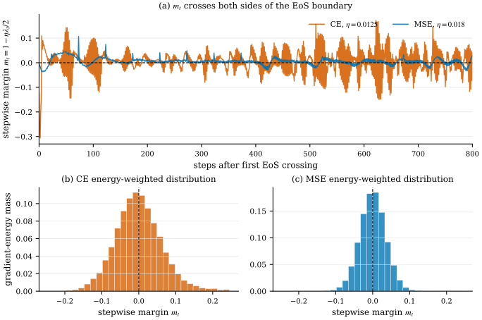
Representative EoS window plots showing repeated sign changes in pointwise margins and their gradient-energy-weighted distributions.

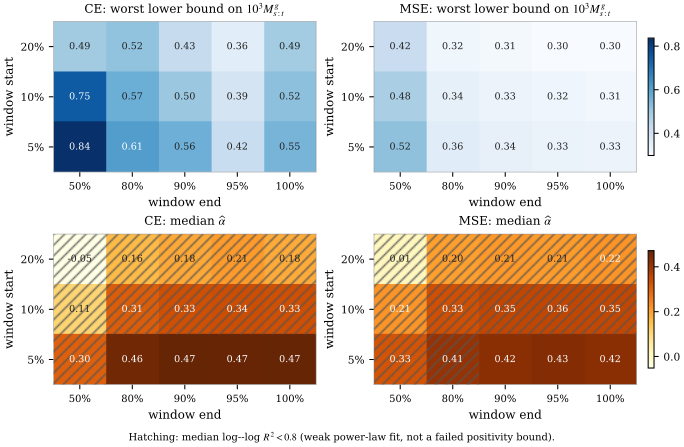
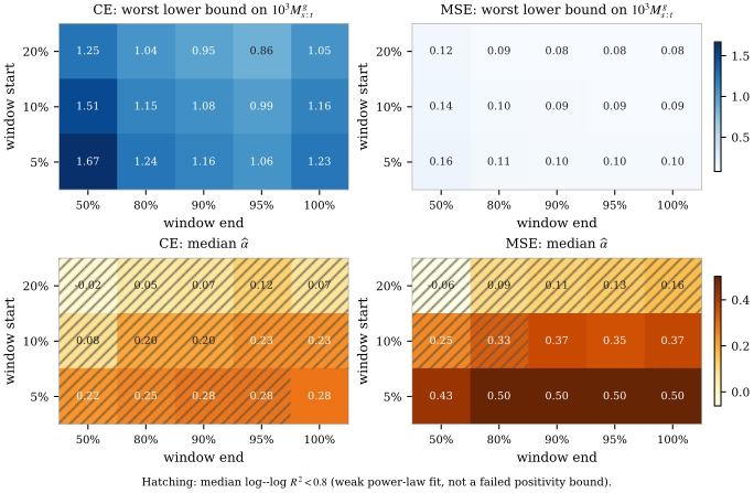
Window-origin sensitivity

ViT

ViT sensitivity of the terminal certificate and inverse-log shape audit to the window origin.

MLP

MLP sensitivity of the terminal certificate and inverse-log shape audit to the window origin.

N:=T-s,\qquad {\color{#557D66}{M^g_{s:T}}} \gtrsim cN^{-\widehat\alpha} \quad\Longrightarrow\quad N{\color{#557D66}{M^g_{s:T}}} \gtrsim cN^{1-\widehat\alpha}.

\widehat\alpha_{\mathrm{median}}\le\frac12 \quad\Longrightarrow\quad \frac1N\sum_{t=s}^{T-1}\lVert g_t\rVert^2 \le \frac{f(x_s)-f_\star} {\eta\,{\color{#557D66}{M^g_{s:T}}}\,N} = O\!\left(N^{-1/2}\right).

M^g_{s_r:s_r+q} \stackrel{?}{\approx} \frac{A}{\log(1+q)}.

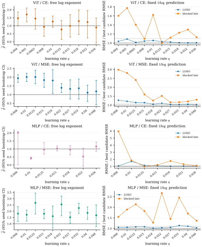
ViT inverse-log diagnostics: free-exponent intervals and normalized predictive errors for cross-entropy and mean-squared error.

MLP inverse-log diagnostics: free-exponent intervals and normalized predictive errors for cross-entropy and mean-squared error.

403eligible post-EoS trajectories

37architecture–loss–rate conditions

0 / 37pass the complete fixed-law rule

Progressive sharpening across the top-10 Hessian spectrum

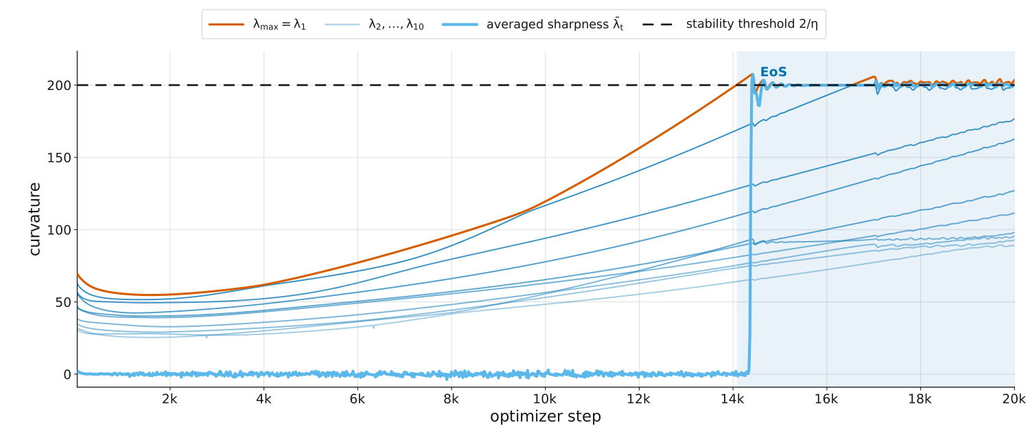
The ten leading Hessian eigenvalues progressively sharpen during full-batch MLP training. The maximum eigenvalue reaches the dashed stability threshold at step 14,080. The thicker sky-blue update-averaged sharpness then oscillates around the threshold in the shaded Edge-of-Stability region.

2-layer tanh MLP, width 200 · CIFAR-10 (50k) · MSE · full-batch GD · \eta=0.01 · seed 1